Histograms
Introduction
What is a Histogram?
The histogram is a tool that visually represents the distribution of brightness values (pixel intensities) of an image. On the X-axis, you see the possible intensity values – for grayscale images from 0 (black) to 255 (white), for color images separately for each color channel (red, green, blue). The Y-axis shows how many pixels in the image have each of these values.
The histogram relates to the entire image. You do not need any prior knowledge in image processing to understand the basic principle: The histogram shows you how "bright" or "dark" your image is overall and how the brightness is distributed.
What is a histogram used for?
The histogram allows you to see at a glance:
How the brightness is distributed in the image (e.g., evenly, predominantly dark or bright)
Whether your image is over- or underexposed (too many very bright or very dark areas)
How high the image contrast is (difference between the brightest and darkest areas)
The histogram is especially helpful during commissioning, selecting and optimizing lighting, fine-tuning exposure, as well as setting thresholds and filters. It supports you in specifically improving image quality.
The histogram provides no information about:
Image sharpness or focus
Geometric errors (e.g., distortions, positional errors)
Content recognition (e.g., object classes, text recognition, specific error types)
Other tools are available for these tasks.
Display & Operation in the Workflow
Where can I find the histogram in the workflow?
The histogram is available to you in the workflow as its own tab – directly next to the "Event Graph" tab. The prerequisite is that a workflow is active and an image has been loaded into a variable of type Image. You do not need to activate the histogram separately, as it appears automatically as soon as an image is present.
Initially, a message is displayed in the tab. This message is always shown when no image is present, for example due to the selection of a variable with an incompatible type - type Image is required.
How is the histogram structured?
X-Axis: Displays the intensity values (0–255 for grayscale, 0–255 per channel for RGB).
Y-Axis: Indicates the number of pixels per intensity value.
Display: Depending on settings, shown as filled area, bars, or lines.
Grayscale Histogram: One channel, ideal for brightness and contrast.
RGB Histogram: Three channels (Red, Green, Blue), displayed separately or overlaid – useful for analyzing color casts or lighting colors.
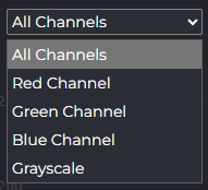
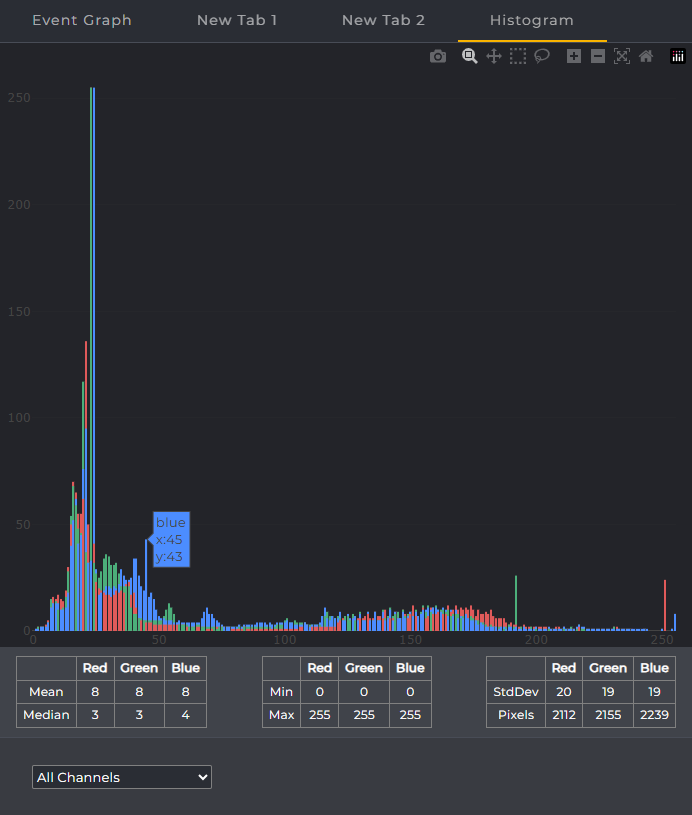
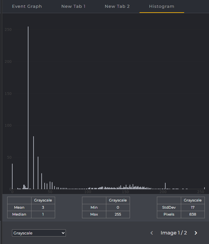
You can conveniently select the desired channel via a dropdown menu. If you have selected a variable of type Image as an array, you can also switch between the images contained in the array in the bottom bar next to the channel selection.
What do the histogram parameters mean
In the lower image area, automatically calculated parameters for the currently selected channel (Mono or R/G/B) and the viewed area are summarized. These values help to objectively classify brightness and contrast and to check changes in exposure, lighting, or filters.
Value | Description |
|---|---|
Minimum (Min) | Smallest occurring intensity value in the selected range. |
Maximum (Max) | Largest occurring intensity value in the selected range. |
Mean / Average | Average intensity of all considered pixels. |
Median | 50% quantile of the intensity distribution (half of the pixels lie below/above). |
Standard Deviation | Measure of dispersion (indicator for contrast). |
Pixels / Pixel Count | Number of pixels included in the calculation (entire image or ROI). |
Additional Tools within the Histogram Tab
When you hover the mouse over the histogram, you will see a list of icons at the top. Among others, the following tools are available to you there:
Tool | Description |
|---|---|
Download Plot as a PNG | Saves the current histogram view as a PNG file (screenshot of the plot). |
Zoom | Enables zooming: Drag a region with the mouse to zoom into that area. |
Pan | Moves the view: Drag the plot to shift the visible area. |
Box Select | Rectangular selection: Select data points within a rectangular area (if supported by the plot). |
Lasso Select | Freehand selection: Select data points with a freeform outline (if supported by the plot). |
Zoom In | Gradually enlarges the view. |
Zoom Out | Gradually reduces the view. |
Autoscale | Automatically scales the axes so all relevant data is optimally visible. |
Reset Axes | Resets the axes/view to the original or default view. |
Many actions, such as Box Select, can be undone by double-clicking. On the other hand, zooming into a selected area is also possible using the left mouse button.
Interpretation & Usage
How do I interpret typical histogram shapes?
Values far left: The image is overall dark (possibly underexposed).
Values far right: The image is very bright (possibly overexposed).
Narrow distribution: Low contrast, the image looks dull.
Wide distribution: High contrast, many brightness gradations.
How does the histogram support my configuration?
The histogram helps you optimally adjust the exposure (time, gain) and the lighting (intensity, direction). You can also specifically set and verify thresholds and filter parameters based on the visible peaks and distributions.
Typical workflow:
Capture image → check histogram → adjust parameters → capture image → check again, until the desired result is achieved.
What does usage look like in practice?
In the displayed histogram, the focus of the distribution is clearly in the midtone range; the curve shows the highest peak there. In the very dark as well as the very bright areas, only low frequencies are visible – neither on the left nor the right is any significant clipping detectable. The overall distribution is moderately wide, indicating a balanced but not extreme contrast.
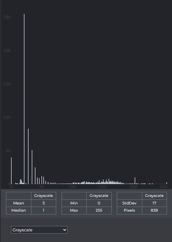
It follows that the motif primarily uses midtones; shadows and highlights are present but without harsh extremes. The exposure appears overall harmonious, with reserves at both ends providing room for slight contrast enhancement without losing details in shadows or highlights.
Advanced Histogram Operations
Histograms are not only used for display and interpretation but can also be actively processed further: for example, for normalization or equalization to improve contrast, for segmentation and feature detection via back-projection, or for comparison/matching of images. The following links lead to practical methods and show how these steps can be applied in the workflow.